Reports with R Markdown
Making plots and being able to write output files is important. However, the most important part of any analysis is communicating your findings effectively! The rmarkdown package is one of the best and easiest ways of doing this. It let’s you create a fancy looking report without ever leaving RStudio. You can interleave your code and plots together with explanation text and formatting you might normally do in a tool like Microsoft Word. You can even make websites with it (like this one!)!
Let’s get started with R Markdown and make ourselves a sweet report.
Creating an R Markdown notebook
In RStudio, go to File -> New File -> R Markdown. It will ask you what you want to call the file - leave the output as HTML for now.
You should see a file open with a lot of text and code already there. This is the default R Markdown document and comes with a lot of pointers about how to do things. For now, save the file as example.Rmd, and hit the “Knit” button.
If everything went well, you should see a nicely formatted webpage/ report pop up in RStudio’s built-in browser. Congratulations, you’ve made your first report!
Basic formatting
Now that we know everything’s working, let’s start from scratch and learn how R Markdown works step-by-step. The first thing we should do is delete everything except for the following:
---
title: "test"
author: "Jeff Stafford"
date: "August 20, 2017"
output: html_document
---
The stuff between the ---s is called YAML - it’s a markup format that describes what kind of document to make, who wrote it, and other technical bits that’s not actual content in your report. If you want, you can modify it, but let’s leave it be for now.
At the bottom of the document, let’s start typing some text. Everything that follows is example markdown output and syntax:
Normal characters result in normal text.
*this makes italics*
**big bad bold text**
***italic AND bold***
# A header
## A smaller header
### An even smaller header
Horizontal lines can be made with lots of dashes. Like this:
----------------------
To start a list, we can use asterisks:
- * Item one
- * Item two
- * Item three
- indenting four spaces makes a nested list
We can make a numbered list by just typing 1. 2. 3.
- first
- second
- third
To make a block of code-y looking text, we use backticks:
`some code`
```
Three backticks makes
a block of text
look the same way.
```
A hyperlink looks like [link text](www.some-website.ca)
Images are just a link with an ! in front:

Some notes on formatting
Text on subsequent lines gets treated as the same line. To have text appear in a separate line/paragraph, you need a blank line in between.
Including code, data, and plots
To include code in a report, we just change the “code” styling slightly. Add a {r} after the triple backticks to have that block of text get treated as R code. The top of the code header should look like this: ```{r}
In practice, it looks something like this:
5 + 6## [1] 11print("The code output gets put directly below")## [1] "The code output gets put directly below"If you want to display data, you have a couple options. The first, is just to print out data the way you normally would.
library(gapminder)
head(gapminder)
## country continent year lifeExp pop gdpPercap
## 1 Afghanistan Asia 1952 28.801 8425333 779.4453
## 2 Afghanistan Asia 1957 30.332 9240934 820.8530
## 3 Afghanistan Asia 1962 31.997 10267083 853.1007
## 4 Afghanistan Asia 1967 34.020 11537966 836.1971
## 5 Afghanistan Asia 1972 36.088 13079460 739.9811
## 6 Afghanistan Asia 1977 38.438 14880372 786.1134However, there is a special function knitr::kable() that inserts a nice-looking table into your report. Depending on what your output format is, it sometimes is even interactive!
knitr::kable(head(gapminder))| country | continent | year | lifeExp | pop | gdpPercap |
|---|---|---|---|---|---|
| Afghanistan | Asia | 1952 | 28.801 | 8425333 | 779.4453 |
| Afghanistan | Asia | 1957 | 30.332 | 9240934 | 820.8530 |
| Afghanistan | Asia | 1962 | 31.997 | 10267083 | 853.1007 |
| Afghanistan | Asia | 1967 | 34.020 | 11537966 | 836.1971 |
| Afghanistan | Asia | 1972 | 36.088 | 13079460 | 739.9811 |
| Afghanistan | Asia | 1977 | 38.438 | 14880372 | 786.1134 |
You can put code inline in text by just typing “r some code” in backtics.
Plots are done the same way as code:
library(ggplot2)
ggplot(gapminder, aes(x=year, y=lifeExp, group=year)) +
    geom_boxplot()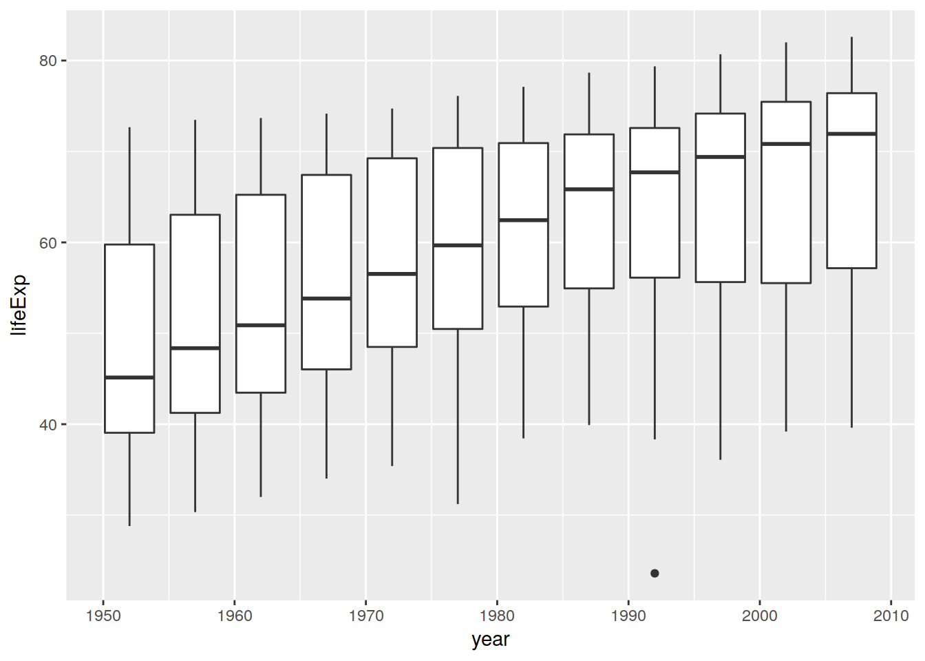
Exercise - Writing your own report
Using any dataset you want, find something interesting and write a report on it in RMarkdown (nycflights13 is a good starting point).